Constant-time algorithm for parametric curves

Behind that seemingly barbaric title is an algorithm that is very useful, and not very difficult to understand.

In computer science, specifically when designing algorithms, the programmer wants to have something that executes fast and uses as little storage as possible (of course). However in most cases you can’t have the best of both worlds : either your process is going to be fast, or it is going to be light on memory, but not both. This is called the space-time tradeoff (or time-memory tradeoff), and can be expressed in very formal and obscure terms by theoretical computer science (as a branch of mathematics).

The truth is that nowadays, computer memory is available in big enough quantities that at least for us game developers, it is nearly always a good idea to go for speed over memory usage – emphasis on “nearly always” – because the computer will “nearly always” have the amount of memory you’ll need. We are now going to see one such case of an algorithm that executes very fast by using lots of memory.

The problem

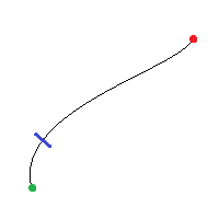
Let’s say you have a curve, and you want to move a point along that curve. It can be something like an enemy going down a complicated path in a shoot-them-up, or plotting a path in a painting program.

Mathematical positioning

A point travelling on a curve

Now comes the problem to define what that curve is going to be. There are several possible methods, but we will chose the parameterization method. A parameterized curve is simply a function which to some real number between 0 and 1 associates a point in space. To put it simply, you can think of the parameter as the percentage of the curve : a value of 0 is the very first point, and a value of 1 is the very last point, while moving from 0 to 1 makes the point go along the curve.

To keep it simple, we will simply look at planar curves, that is, curves that lie in a simple 2D plane. Thus, we can define our planar curve like so :

From that definition, the entire curve is simply .

This definition however isn’t really adapted to game development : as curves get spatially complex (with lots of loops, fancy movements etc), their parameterization formulae get equally intricate, and sometimes simply evaluating them for a known parameter becomes a problem due to the sheer computing power needed, especially if you need to do it a lot of times per frame. So what we do instead, is we sample the curve along a fixed timestep.

Fixed timestep sampling and the travel speed problem

So let’s take our planar curve in the form of its parameterization , and let’s put it in a form more suited to game development : a simple array of elements. We do that by taking a finite number of values for our parameter and storing the (equally finite) values of in the array. The number of samples we take depends on the precision we want (and the amount of memory we are ready to take up). The formula is simple ; for , you can take samples with :

Sampling of a curve with 20 samples (shown as red dots).

 

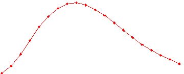
for i = 0 to k:
  array[i] = f(i / k)

The resulting array is called a sampling of the curve, and to use it, you simply perform linear interpolation on its values. Geometrically speaking, this is the same thing as linking all your red dots with a straight line : it’s not exactly your initial curve, but it’s close enough, and the computations are much simpler. In the above image, we sampled the curve with 20 samples, corresponding to the values of for = 0, 0.05, 0.1, 0.15 … 0.9, 0.95, 1.

But then a problem arises : we see on the image that the points are not at the same distance from each other. In other words, the first point is closer to the second point than the second point is to the third, and so on in an unpredictable manner. This is due to the slope of the curve, and a bit of differential geometry will tell you that the steeper the curve is, the closer successive sampling points will be, and that the flatter the curve is, the more distant successive points will be. This is a problem to us, because this means that the travel speed on the curve is not constant, and actually depends on where on the curve we are. Instead, we want to make sure that a point traveling on the curve does so at a constant speed, regardless of where it is on the curve (formally speaking, we want the norm of the derivative of the curve to be a constant).

An example is as follows : say an enemy is moving on the curve of the above image, and must complete it in one second. It starts at t = 0 at the point and ends at t = 1 at the point , and of course you want it to have a constant velocity. The problem is that the enemy travels a greater distance between the second and the third point than between the first and the second, although both took the same duration (namely 0.05 s, one twentieth of a second) ; thus its speed is not constant.

The arc length parameterization

To solve this problem, we look at a new parameterization : the parameterization by arc length.

Sampling of the arc length parameterization : here, every point is at the same distance along the curve to its neighbours as every other point

Unlike the naive parameterization that we have been using up until now, which most of the time is made of polynomial functions of the parameter t (ie sums of powers of t), the arc length parameterization is, by definition, a solution to the travel speed problem. It is defined as a function that to a real number between 0 and 1 associates the point of the curve that is at s% of the total length of the curve. So for example, for the corresponding point is the one in the middle of the curve.

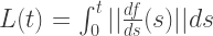
There is a formula giving the arc length along the curve from the origin of the curve to a point given its t parameter for any (differentiable) curve :

Finding the arc length parameterization is equivalent to reversing the above equation to get t as a function of L. But as you can see, it is very hard to calculate by hand for arbitrary curves, and even more so with an efficient algorithm that is suitable to game development, so instead we will again calculate a sampling of this parameterization, but this time by looking at things in reverse.

Reverse sampling of the arc length parameterization

This algorithm allows one to perform constant-time () curve lookups for any parameterized curve (and any parameterization), that is, the amount of time taken to calculate for any value of is independent to the number of samples in the sampling of the curve, and thus independent of the precision of the sampling !

The idea of the algorithm is to hold an array of samples, just like before, and an array of indices into the array of samples. The trick is that the array of indices is ordered in such a way that it actually solves the travel speed problem.

To illustrate the situation, let’s look at our arrays like we look at mathematical functions. Before, we had the and parameters, which are respectively the arc length and naive parameters. The indices array is like a function so that , so it maps our arc length parameter to the corresponding naive parameter values, and it does so in constant time (simply an array lookup). Now that we have , we can now use the samples array to do a curve lookup, again in constant time !

The only tricky bit lies in how the indices array is constructed. The algorithm is as follows, for with k+1 samples :

lengths[0] = 0
samples[0] = f(0)
for i = 1 to k:
  samples[i] = f(i / k)
  # approximate curve length at every sample point
  lengths[i] = distance(samples[i], samples[i-1]) + lengths[i-1]
# normalize lengths to be between 0 and 1
lengths = lengths / lengths[k]

indices[0] = 0
for i = 1 to k:
  s = i / k
  j = so that lengths[j] <= s < lengths[j+1]
  indices[i] = j

The algorithm lies in this simple idea : given s the arc length parameter, you can easily find the two consecutive samples of respectively lesser and greater distance to the origin than s ; this is what the lengths array is for. Once you have found the index of the first sample (the other index is the same + 1), it also happens to be the index in your samples array of the correct sample. A little bit of linear interpolation just like before is clearly enough to give you the correct point on the curve ! This is all made into a constant time algorithm by the use of the indices array, which does require an array search ( with a binary search) to be constructed – but only once !

After those arrays are constructed, the following code can be used, given an arc length , to find the corresponding point on the curve :

function curve(s):
  i = floor(s * indices.length)
  t = indices[i]
  point = lerp(samples[t], samples[t+1], s * indices.length - i)
  return point

where is the linear interpolation between a and b of value x.

Ending word

This concludes the article on constant-time curve lookup. I don’t think this can be greatly optimised, as constant complexity is indeed the optimal case for any algorithm, but if I missed anything please do let me know. Also if you have any question on the algorithm itself, I’ll be happy to answer them, be it in the comments or by mail (see the Contact page).

I will try and wrap up a quick working demo of this algorithm in Haxe, which is a language that is high-level enough to be understood simply. This will be the subject of another article, so look out for that !

Matrefeytontias